Jones PD , Raper SCB, Goodess CM,  Cherry BSG,  Wigley TML,   (1986)  TR027  A Grid Point Surface Air Temperature Data Set for the Southern Hemisphere. Office of Energy  Research , Carbon Dioxide Research  Division, US Department of Energy. Under Contract No. DE-ACO2-79EV10098

ABSTRACT

A compilation of 610 station records of monthly surface air temperature has been assembled for the Southern Hemisphere, north of 62.5° S.  In order to use these data to construct the first grid point temperature data set for the Southern Hemisphere, the homogeneity of each of the station records has been assessed.    Each station has been classed into one of these groups;  immediately usable, corrected or uncorrectable.   The results are presented in tabular form.
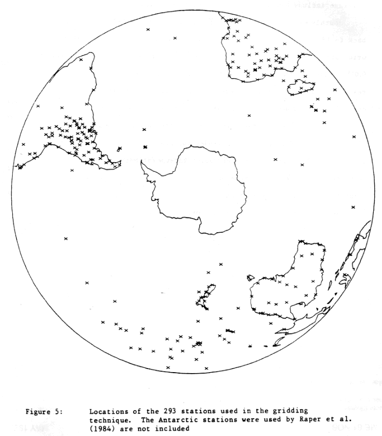
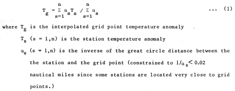
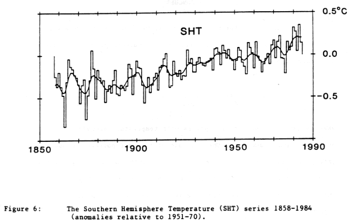
Of the 610 station records, 293 were used to produce a gridded data set on a 5°  latitude by  10°   longitude grid between 5°  S and 60° S inclusive.    Grid point anomalies for 1851 – 1984, with respect to the reference period 1951-70, were interpolated from station data using a simple algorithm.   In order to produce a best possible data set, Antarctic data were included after they became available in 1957.


TABLE OF CONTENTS
                                      
Abstract  
Table of Contents    ii
Acknowledgements   
Introduction     
Station Homogeneity Assessment     
Gridding the Station Data    
Conclusions    
References
Appendix A:    Station History formation and Homogeneity
    Assessment Details    
Appendix B:    Stations used in the Gridding Algorithms    

ACKNOWLEDGEMENTS
The work described in this Technical Report was funded by the U.S Department of Energy under Contract No. DE-AC-79EV10098 and Grant No. DE-FG02-86-ER60397.

INTRODUCTION
Although many studies have been undertaken with temperature time series purporting to represent the whole globe, most are only representative of conditions over the Northern Hemisphere land masses. A truly representative average for the whole globe can only be achieved by incorporation of data from both the land and marine area of both hemispheres.
Early studies by Willett (1950) and Mitchell (1961) using land-based data from both hemispheres indicated that a reasonable proxy for global conditions could be formed from age for the Northern Hemisphere land mass only. Indeed, this was a convenient supposition to make, because data for the Northern Hemisphere land masses are the most plentiful and readily available. In support of this supposition it has been argued that external forcing factors should affect the hemispheres similarly, in both degree and timing. However, the representativeness of the Northern Hemisphere land data in a global context can be questioned because the number of Southern Hemisphere stations used by Willett and Mitchell was small, only one fifth of those used for the Northern Hemisphere with almost all been located between the equator and 40° S.
Recent work by Folland et al. (1984) using marine data has shown that important differences are apparent between the land and marine records for the Northern Hemisphere (Jones et al, 1986a) and between the marine records for the two hemispheres. The differences are most apparent in the degree of warming and cooling during the present century (see Wigley et al., 1985, 1986)
A detailed study of the hemispheric temperature trends for the Southern Hemisphere will enable more detailed comparisons of the Northern and Southern Hemisphere land and marine data sets to be made. The land areas of the Southern Hemisphere have often been ignored in previous studies; the only recent analysis to consider this region comprehensively being that of Hansen et al. (1981)

Data Sources
The basic source of station air temperature data for the Southern Hemisphere land masses in the set of volumes of World Weather Records (WWR) (Smithsonian institution, 1927, 1934, 1947, and U.S Weather Bureau, 1959-1982; available in digitized form from the National Center for Atmospheric Research (NCAR), Jenne, 1975). A considerable amount of additional temperature data for Argentina and Chile for the years 1931-60 has recently been added to this set. In WWR, these countries only have data available from 1951 (see Pittock, 1980, for further details).
Searches for data in archives as part of the present project yielded additional data for Indonesia
and Australia and for some Pacific Islands, particularly Tahiti. Additional data for New Zealand was found in Salinger (1981). For Peru, the Peruvian Meteorological Service supplied information for about 10 stations covering the 1940s and 1950s. Additional data for Australia was provided by their Bureau of Meteorology. All of these sources are gratefully acknowledged.
Altogether 610 stations (between 2°.5 S and 62.5° S) were used in this analysis. The names, locations, elevations and record lengths of all 610 stations are listed in Appendix A
For the Antarctic region we used the data given in Raper et al. (1984) and updated in various issues Climate Monitor.

STATION HOMOGENEITY ASSESSMENT
It has long been known that the basic source of temperature data, World Weather Records, contains many records that are not homogenous. Furthermore, we assumed that a significant fraction of the new station data could be non-homogenous, although Salinger (1981) has inspected and corrected most of the New Zealand data. Station data may contain the effects of changes that result from non-climatic factors (see Jones et al., 1985, 1986a, and Bradley and Jones, 1985, for a list of these factors and examples of their effects). The composite Southern Hemisphere data set was therefore analysed for homogeneity in a manner similar to that for the Northern Hemisphere (Jones et al., 1985).or each of the 610 stations in this data set, data homogeneity was assessed, where possible, by comparing each station record with neighbouring station data. The technique is outlined in Jones et al. (1986a). When identified, inhomogeneities were corrected by comparison with neighbouring station data in a manner described by Jones et al. (1985).
Four examples of the homogeneity assessment are shown in figures 1 to 4, each been discussed in the appropriate figure caption. The examples are:
Fig. 1, Curtiba (WMO No. 83842) minus Rio de Janeiro (837430) (Brazil)
Fig.2 Ushuaia (879380) minus Punta Arenas (859340) (Argentina-Chile)
Fig.3 Johannesburg (683697) minus Durban (685880) (South Africa)
Fig.4 Lauthala Bay (916900) minus Nandi (916800) (Fiji)
Further examples are given in Jones et al. (1986b)
Details of this assessment are listed in Appendix A, which includes reference to some of the neighbouring stations used for comparisons, corrections applied, (if any) and station history information. The format of this Appendix is exactly the same as given in Bradley et al. (1985) and Jones et al. (1985).

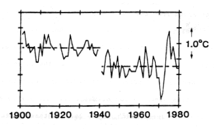
Figure 1:  Station temperature difference time series: Curitiba (25.4S,  49.3W) ,minus  Rio de Janiero (22.9S,  43.2W) 1901-1980.  The analysis identifies Rio de Janiero as the errant station as a similar jump at 1941 also occurs when the station is compared with Iguape (24.7S, 47.5W). The station history information reveals that the observation time and station height were altered around 1940.  The straight lines are the mean station differences for the two periods, 1901-1939  and 1941-1980. Correction details are given in Appendix A.

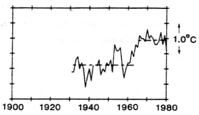
Figure 2:  Station temperature difference time series: Ushuaia (54.9S,  68.4W) ,  Punta Arenas (53.3S,  70.9W), 1931-1980.  The analysis identifies Punta Arenas as the errant station as a similar jump at 1963 also occurs when the station is compared with Rio Gallegos (51.6S, 69.4W).   A change of station site is indicated because of a data gap around 1963. The straight lines are the mean station differences for the two periods, 1931-1963  and 1964-1980. Correction details are given in Appendix A.

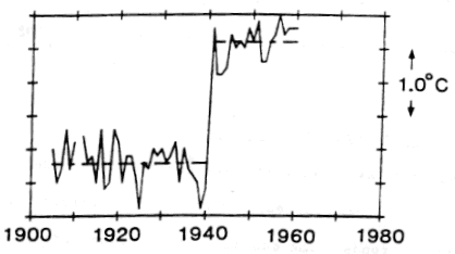
Figure 3:  Station temperature difference time series: Johannesburg  (26.2S,  28.1W) ,minus  Durban (29.9S,  31.0W) 1905-1960.  The analysis identifies Durban as the errant station as a similar jump at 1941 also occurs when the station is compared with Aliwal North (30.7S, 26.7W). The station history information reveals that the station was moved to the airport in 1941.  The straight lines are the mean station differences for the two periods, 1905-1940  and 1941-1960. Correction details are given in Appendix A.

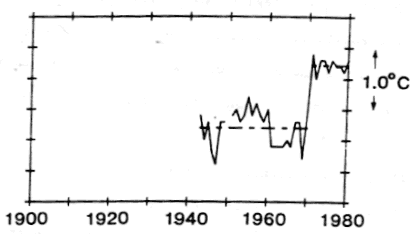
Figure 4:  Station temperature difference time series: Lauthala Bay  (18.1,  178.4W) ,minus  Nandi (17.9S,  177.5W) 1943-1980.  The analysis identifies Nandi as the errant station as a similar jump occurs when the station is compared with Oni-I-lau (20.8S, 178.8W). The station history suggests a change of observation times after 1971.  The straight lines are the mean station differences for the two periods, 1951-1940  and 1971-1980. Correction details are given in Appendix A.

Results of the Station Homogeneity Assessment
Each station has been assigned a quality control code, identifying records which are correct, homogenized, uncheckable, incorrect, or affected by non-climatic warming trends. The quality control codes are given in Appendix A. In some instances ‘correct’ stations are only correct after a specified year – the first reliable year. In these cases earlier data are suspect and could not be reliably checked. These early data have not been used to derive grid point anomalies.
The number of stations in each homogenization category are listed in Table 1 for the three main continental regions of the Southern Hemisphere: southern Africa, South Africa, and Australasia. Island stations are associated with the appropriate WMO region (i.e. Africa includes stations south of 2.5 S with WMO identifiers commencing with a 6, South America includes stations between 2.5 S and 62.5 S with WMO identifiers commencing with a 9).
The number of stations which cannot be checked is roughly 46% of total. Most of these records are too short for the homogenization analysis, generally having less than 20 years of data. Over half of these stations are located in South America, especially in Brazil. The lack of Brazilian data has been highlighted in Jones et al. (1986b) The proportion of incorrect

stations which could not be corrected is considerably smaller than for the Northern Hemisphere (Jones et al., 1985), although this was not a problem in the Northern Hemisphere because of the greater total number of stations.
In order to average the station data to produce regional and hemispheric mean values it is necessary to reduce all the monthly station data to anomalies. This eliminates the effect of different station elevations and other factors. The period with the best data coverage, 1951-70, has been used as the basic reference period. The numbers of correct and homogenized data with sufficient reference period data (at least 15 of the 20 years between 1951 and 1970) for the three regions are listed in Table 2. A few stations with a long period of record, but without adequate reference period data have been included. For these stations, reference, period means were estimated by comparison with neighbouring stations. The accuracy of this estimation is ±0.2 C.
Altogether 293 stations were used in subsequent analyses. The names, locations and years of operation of these stations is listed in Appendix B. The locations of the 293 stations are shown in Figure5.   Further discussion of the station homogeneity assessment is given in Jones et al. (1986b).

In order to overcome the irregular spatial distribution of the station data, we have interpolated the data onto a regular 5  latitude by 10  longitude grid. This is exactly the same grid spacing as used for the Northern Hemisphere by Jones et al. (1986a) and Vinnikov et al. (1981). As was noted earlier, it is necessary to reduce all the station data to anomalies because of different station elevations and to a lesser extent, different observation times. The reference period used was 1951-70.
Each station was associated with its nearest grid point in terms of great circle difference. Grid-point departures (from the 1951-70 reference period) were calculated by averaging all the stations near a point using inverse distance weighting.

The number of stations nearest to a particular grid point varied from grid point to grid point and from one period to another. In many cases only one station was used, and the station value simply becomes the grid-point value. In others, up to ten stations were averaged. Areas of denser station coverage include New Zealand and northern Argentina.
Monthly mean grid point anomalies, relative to 1951-70, were calculated back to 1851 for all possible grid points between 5 S and 60 S inclusive.
Grid points anomalies have been calculated and are stored to an accuracy of 0.01 C, although this does not reflect the accuracy of the original data. The results are not particularly sensitive to the method of gridding, as demonstrated in Jones et al. (1986a). Other uncertainties, however, mean that individual monthly grid point anomalies are probably only accurate to ±0.2 C. Our gridded data file includes two measures which can be used to assess the reliability of the grid point interpolations: the number of stations used (n) and the value of                     

These two quantities are given for each month and for each grid point.
The data set is available on a computer magnetic tape.

CONCLUSIONS
Using this particular grid it is relatively easy to calculate an average time series (SH60) for the land areas of the Southern Hemispheres between 2.5 S and 62.5 S

where M is the number of grid points with temperature anomalies (Tg) in a particular month and  g is the latitude of the grid point. The number of grid points incorporated into SH60 increases with time reaching maximum coverage between 1951-1970, during which period approximately 27% of the entire Southern Hemisphere can be gridded (i.e. 30% of the 2.5-62.5  region).
The effect of less complete coverage prior to 1951 has been assesses by Jones et al. (1986b). This assessment was carried out by comparing hemespheric estimates based on a sequence of frozen grids (viz. grid points available for each decade between the 1850s and 1930s) with estimates based on the best possible grid. Comparisons were made over the period 1941-80. The results indicate that SH60 is a reasonably homogenous and representative time series back to about 1890. Although the series  is undoubtedly less reliable prior to this time, decadal mean values are useful indicators of mean temperatures back to the 1860s.
In order to produce the best possible land average for the entire Southern Hemisphere it is necessary to include Antarctic data. Sufficient data for this continent are only available since  the International Geophysical Year in 1957. The best possible Southern Hemisphere area average, SHT , was calculated using 
SHT = (a(SH60)  +  b (ANT)) / (a + b
where ANT is the Antarctic series produced by Raper et al. (1984), and a and b are the areas of coverage of each series, expressed as proportions of the total Southern Hemisphere area. Although a and b vary slightly with time between 1957 and 1984, a is approximately four times b. Prior to 1956, the best possible Southern Hemisphere land average is simply the SH60 series (i.e. SHT and SH60 are identical).
The SHT series shows little overall trend during the nineteenth century (Figure 6). After 1900, the series shows a warming trend to the mid 1940s. Between about 1945 and 1970 no trend can be seen. Since 1970 a strong warming trend has set in. The three warmest years of the entire record are 1980, 1981 and 1983. The overall warming trend since 1900 is about 0.5 , of which roughly 0.3 C occurred between 1900 and 1945 and 0.2 C since 1970.
The history of land-based Southern Hemisphere temperature series is, therefore, not dissimilar to that for the Northern Hemisphere. However, the early twentieth century warming up to 1940 is smaller in magnitude and the cooling evident in the Northern Hemisphere between 1940 and 1965 appears only as a hiatus in the longer-term warming trend. Further discussions of this data set and comparisons with the marine data for the Southern Hemisphere are given in Jones et al. (1986b)